The Detailed propagation course

HTML Propagation Fundamentals - Fixed Link Propagation - Mobile Propagation

PDF Fixed Links Propagation - Mobile propagation

Short and simple (the old tutorial)

Propagation in Free Space - Absorption by Atmospheric Gases - Diffraction over Terrain - Refraction and Ducting - Reflections - Troposcatter - Rainscatter - Sporadic E

Reflections from the Ground

The reflection co-efficient for ground reflections depends principally on the dielectric constant e and the conductivity s. It is different for vertical and horizontal polarization.

Figure 1 - Reflection Geometry

The resulting reflection coefficients are given by the equations below:

Note that in general the reflection co-efficient is a complex number and the reflected signal with therefore differ in both amplitude and phase. Making substitutions for complex permitivity and complex permeability gives the complex reflection coefficients:

For small q, r => 1, for q => 180, r =>-1

The table below gives some typical values which are plotted in Figure 2.

Figure 2 - Reflectivity over Ground

Figure 3 - Reflection Phase Change

Reflection from rough surfaces

The reflections from rough surfaces are termed non-specular reflections.In general the resulting reflection from a real surface will be a combination of specular and non-specular reflections as shown in Figure 4.

Figure 4 - Reflections from Rough Surfaces

But how is a rough surface defined? The relative smoothness of surface depends on:

• Wavelength
• Angle of incidence

It is common to employ the “Rayleigh Criterion”. In figure 5 there is a different path length for both rays of 2dsin(Y) and the phase difference is this length multiplied by 2p/l.

Figure 5 - Rayleigh Criterion

for a rough surface. Typically, roughness is described by the standard deviation of the surface around the mean, s. A constant is derived measuring the roughness:

The Rayleigh criterion is C < 0.1 for a smooth surface. If C > 10 then the reflection is so diffuse it can be neglected.For example, at an angle of 30 degrees at 1.6 GHz, a rough surface has a s of more than 3mm. At 5 degrees it is 1.8cm.

The Rayleigh criterion can only be a guide, in general the angle of incidence will vary as surfaces are not in general parallel unless man made to demonstrate reflections in physics experiments.

Scattering from Real Objects

In the real world there are likely to be many more than 2 rays to be summed from multiple scatterers and these will be of arbitrary or at best unknown phase. These objects may be raindrops in the atmosphere, trees, terrain, buildings, aircraft etc etc. The best option here is to sum the power.

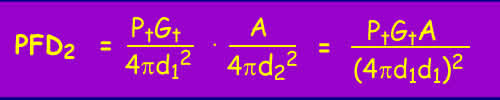
Recall from the free space loss tutorial that the power flux density at a distance d1 from a transmitter of power Pt with antenna gain Gt is given by:

The scatterer is assumed to have an effective area A and to re-radiate all the energy it receives isotropically, that is equally in all directions. Therefore the scattered power flux density at some further distance d₂ is:

At the receiver antenna the power received is the gain of the antenna multiplied by its effective aperture (l² / 4p).

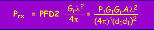
The "path loss" is the ratio of the transmitted to received power. Path loss can be a confusing term, as it is not really a loss at all but a measure of what proportion of the signal is lost on the trip. It might be more accurate to call it a path gain, or to plot the value P_tx/P_rx instead, but this would only add to the confusion. A path loss of 1 means all the energy is transferred and a path loss of say 0.01 means only 1% gets through¹.

Which is better known as the bistatic radar equation. Note how it includes the antenna gains, so don't go adding these twice by working with the EIRP or adding the receiver antenna gain. For a normal Radar, the transmit and receive antenna gains are the same, as are d₁ and d₂ which are usually called the range, as in RADAR = RAdio Detection And Ranging.

Trying a few figures for example, at 10 GHz radar with a wavelength of 0.03m with a scatterer of area 0.0001 m² (1 cm²) and the range being 100 000 m the "path loss" for a 50dB gain antenna (G = 100 000) is 4.5x10^-21 which is -203dB. With a transmitter power output of 100kW (50dBW) the received power is 0.00045 picowatts, which is - 153dBW. A typical receiver sensitivity with averaging is around this value, so is a good chance of detecting this scatterer.

Radars are frequently used to detect raindrops. The Chilbolton Radar is an example of a weather research radar, it operates at 3GHz using 600kW pulses to a 25m dish with 53dB gain and can detect light rain at over 100km range. Raindrops have an area of the order of 1sqmm. The equation above demonstrates why such a large installation is necessary.

The next section of this tutorial deals with scatter based propagation mechanisms.

Notes:

¹Usually these values are expressed in decibels, 10log₁₀(value). Decibels are simply ratios expressed logarithmically to make the numbers easier to handle. If the ratio is relative to some standard, then that unit is appended, so for example dBW is power relative to one Watt and 0 dBW = 1 Watt and 10dBW = 10W.

© Mike Willis December 26th, 2006