The Detailed propagation course

HTML Propagation Fundamentals - Fixed Link Propagation - Mobile Propagation

PDF Fixed Links Propagation - Mobile propagation

Short and simple (the old tutorial)

Propagation in Free Space - Absorption by Atmospheric Gases - Diffraction over Terrain - Refraction and Ducting - Reflections - Troposcatter - Rainscatter - Sporadic E

Diffraction is a large subject with some fairly difficult mathematics - the intention here is just to cover the basics. Skip the equations if you like.

Consider figure 1 - a plane wave comes across an obstruction, the energy above the obstruction passes and the rest is blocked. This does not happen in reality and the reason is diffraction. Figure 2 shows a more likely result.

Figure 1 - Not reality

In reality, there is diffraction around the barrier as shown with some exaggeration in figure 2.

Figure 2 - More like what happens

The Huygens principle of wavelets can be used to explain this - “Each point on a wavefront acts as a source of secondary wavelets. The combination of these secondary wavelets produces the new wavefront in the direction of propagation”.We can express this as an integral:

Where v is the height of the obstruction. Fortunately, this is solvable with a few substitutions:

This is tricky to solve by hand but there is an approximation for v >1

When is Diffraction Significant - Fresnel Zones

An obstruction is generally considered to be significant when it impinges into the first Fresnel zone.

The first Fresnel ellipsoid is bounded by the ellipses where the path length from transmitter to receiver is exactly a half wavelength longer, the second where the path length difference is one and a half wavelengths etc etc. I.e. the area inside the contour where Dl < l/2 is the first Fresnel zone. Dl < 3l/2 is the second etc.

Figure 3 - Fresnel Ellipsoids

Putting it into Practice

The theory above is a simplification, but it is still not practical to apply easily. The result for the signal amplitude after an ideal knife edge is shown in figure 4. This can be used to calculate the diffraction loss as a function of the Fresnel parameter v as defined above.

Figure 4- Knife Edge Diffraction

It is notable that as the knife edge comes into the first Fresnel zone the amplitude rises and then falls fairly linearly, this function can be approximated for v >-0.7 as:

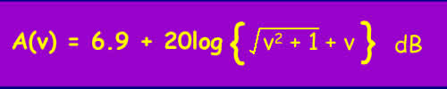
Approximation for Fresnel integral for knife edge

Diffraction around real objects

Most real-world obstructions are large in comparison to the wavelength - i.e. not knife edges. It is possible to solve the equations for idealised cases. Solutions for many objects and including reflection effects, loss from trees etc. rapidly become impractical. Therefore path loss prediction models are used.

There are several models in general these involve adding additional loss to the knife edge loss. Where there are multiple knife edges further models are available, the one currently used by the ITU-R for terrestrial links is a modified version of the Deygout model. More information is available in Recommendation ITU-R P.526 - Propagation by Diffraction. If there is demand, I will include some of the models here. A diffraction model is included in the pathloss software

Frequency

Higher frequencies have shorter wavelengths and therefore smaller Fresnel zones. As a result, as frequency increases for a given partially obstructed path, less and less of the first Fresnel zone is obstructed. However, as the Fresnel zone is smaller, the increase in diffraction loss with increasing obstruction (e.g. as the height of the receiver is lowered) happens much more quickly.

© Mike Willis December 26th, 2006