The Detailed propagation course

HTML Propagation Fundamentals - Fixed Link Propagation - Mobile Propagation

PDF Fixed Links Propagation - Mobile propagation

Short and simple (the old tutorial)

Propagation in Free Space - Absorption by Atmospheric Gases - Diffraction over Terrain - Refraction and Ducting - Reflections - Troposcatter - Rainscatter - Sporadic E

Scattering from Inhomogenities

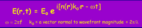
This is what most people mean by Tropospheric scatter. It is the scattering of RF energy from regions of the troposphere with slightly different refractive index. Recall from the tutorial on refraction that the refractive index governs the speed of propagation in a medium:

Although the scattered field is weak, tropospheric scatter is often the dominant mechanism of trans-horizon propagation for the majority of the time. The diffraction field falls off fairly rapidly with distance when there are multiple diffraction points along the path and the other major mechanism of ducting is relatively rare occurring for maybe up to 20% of the time and frequently much less depending on location.

Troposcatter signals vary in amplitude with time. The slow variations are due to changes in the atmosphere and occur on the timescales of hours with a log normal distribution. Typically these variations amount to 10dB on 200km paths overland. Rapid fading is caused by the motion of small irregularities in winds - the scattered signal is a sum of many scattered signals with randomly varying phase which add together. The frequency of variation is of the order of minutes at low VHF (50-70MHz) rising to fractions of a second in the microwave bands. Optical scintillations naturally are much more rapid.

To couple between transmitter and receiver the scattering must occur within a common volume formed by the intersection of the beams of both the transmitter and the receiver antennas.

Modeling Troposcatter

(maths with HTML - what a nightmare!)

The median transmission loss (that not exceeded for 50% of the time) is modeled using ITU-R recommendation P.617.

L50 - M + 30 log f + 10 log d + 30 log q + Ln + Lc - Gt - Gr

Where f is the frequency in MHz, d is the distance along the great circle path from transmitter to receiver measured in km. Gr and Gt are the Receiver and Transmitter antenna gains and the remaining parameters are calculated as follows:

q is the scatter angle in milliradians.

q = qe + qt + qr

Where qt and qr are the transmitter and receiver horizon angles and

qe = 1000 d/Re

Re = effective earth radius ~ 4/3 x 6370km.

The value of M varies between 19dB and 40 dB depending on the climate In the UK the usual values are M=33 dB for overland paths and M=26 dB for paths over the sea.

Ln accounts for the transmission loss variation with the height of the common volume (there is less air higher up).

Ln = 20log(5 +gH) + 4.34gh

Where H = 10^-3 qd/4 and h = 10^-6 q² Re/8 and g is a climatological parameter ~0.27 km^-1 in the UK.

Lc is the aperture to medium coupling loss taking account of the common volume variation with antenna gain:

Lc = 0.07 e^{0.055(Gt + Gr)}

It is possible to calculate for other percentage of time values using a correction factor:

L(p) = L(50 - Y(p)

Where Y(p) = C(p)Y(90)

Y(90) again depends on climate and location

Y(90) = - 2.2 - (8.81 - 2.3x 10^-4 f)e^-0.137h over land

Y(90) = - 9.5 -3e^-0.137h over sea

Going the other way, to lower time percentages down to around 20%, the distribution is symmetrical so:

L(p) = L(50) - {L(100-p) - L(50)} when 20 < p <50

An Example

Frequency 144 MHz, Antenna Gains 16 dBi path length 250km. Horizon angle in both cases = 0 degrees.

q = qe = 1000 x 500 / (1.333 x 6370) = 29.4

M = 32

H = 1.84

h = 0.92

Ln = 15.9

Lc = 0.41

L(50) = 149 dB

Molecular Scattering:

It must be recalled that the energy in a radiowave is quantified into discrete packets of energy called photons - wave/partial duality etc. The energy of the photon is related to the frequency of oscillation e = hf, where h is Plank's constant. When considering the scattering of high frequency radiowaves, it is often more convenient to think in terms of photons.

• Rayleigh Scattering

When photons are of wavelengths comparable to the the size of gas molecules, scattering occurs. The most common mode of scattering is elastic scattering where energy is not transferred from the photon to the molecule. This type of scattering is called Rayleigh scattering. This scattering increases with the fourth power of the frequency, which incidentally is why the sky is blue.

• Raman scattering

It is also possible for photons to interact with gas molecules in an inelastic manner so that energy is transferred between the photon and the molecule. This is called Raman scattering and this is of particular importance to optical communications systems.

At higher photon energies incident photons can excite vibrational modes polarised molecules. This is an energy transfer process with the resultant emission of a scattered photon of lower energy (i.e. lower frequency/higher wavelength) and leaving the molecule in a higher energy vibrational mode. Only certain vibrational mode energies are allowed and by inference, only discrete frequency/wavelength differences can occur. The spectra of the resultant scattered photons forms a set of spectral lines at discrete offsets from the original frequency/wavelength called "Stokes lines". It is also possible for a molecule to give up some of its energy to an incident photon and thereby increase the photon energy. Again, this forms a discrete set of lines, the "anti-Stokes lines".

© Mike Willis December 26th, 2006