Hydrometeors

We will now mode on to Non-clear air, that is air containing rain sleet and snow. Hydrometeors simply mean there is water in the atmosphere.
Forms include Rain, Snow, Hail, Fog, Mist, and Clouds (Ice crystals). As far as the radio wave is concerned, they are bits of lossy dielectric suspended in air. Just like troposcatter there will be scattering but there will also be dielectric losses. Cross polar isolation is also reduced which means less channel capacity.

The Refractive Index of Water and Ice

The refractive index of water is rather complicated with a strong temperature and frequency dependence. The real part is around 10 up to 30GHz with the imaginary part varying from around 0.2 to 2 but generally rising with temperature and frequency. Above 30GHz both the real and imaginary parts fall. http://www.philiplaven.com/p20.html gives an excellent summary.

The low value of the imaginary part of the refractive index of water in the region 1mm to 100nm indicates that water will be transparent at optical frequencies, as we all know, it is.

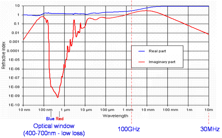
The real part of the refractive index of ice is around 1.78 up to 300GHz with a small imaginary component (loss tangent) that falls with frequency. This is incidentally why microwave ovens are not good at melting ice.

Where is there liquid water in the air?

Much of the water that is in the air is in the form of water vapour rather than as a liquid or solid hydrometeors. As water freezes at 0C, where the air temperature is below 0C the predominant hydrometeors are ice. At just below the height where the temperature is 0C this ice melts and falls as rain - though it is nothing like as simple as that in practice. Ice and liquid water are both heavier then air and the only thing stopping them falling to the ground are rising air currents. As water condenses out of the air it forms ice crystals which are small enough to be supported by rising air currents. These particles clump together and get larger until they are too heavy for air currents to support. These heavy particles fall as rain, hail or snow. There is a fair amount of turbulence associated with clouds and the region where ice is melting into rain and forming large particles is a particularly good scatterer of microwave energy. In weather radars it is described as the bright band as it produces a strong return echo.

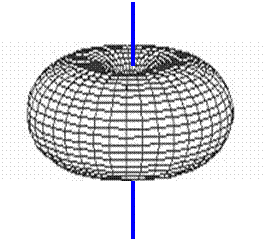
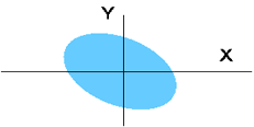
Incidentally, the shape or a rain is nothing like the shape typically drawn in cartoons. That is the drop you get from a dripping tap.

In reality, raindrops tend towards spheres but the force of the air on their base as they fall flattens them into oblate spheroids, the image above is exaggerated. When drops get really large they get more squashed in at the base.

 

Rain Cells

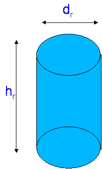
Rain is not uniform but we can approximate a rain storm as a group of rain cells moving over an area. The simplest approximation of a rain cell is a cylinder of uniform rain extending from the cloud base to the ground. There are of course much more complicated models.

Typically h_r is around 3km. d_r ~ 3.3R^-0.08 where R is the rainfall rate in mm/hour. E.g. for Heavy rain, R = 50mm/hr or more, d_r = 2.4km

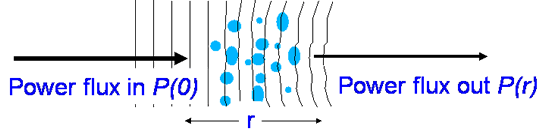
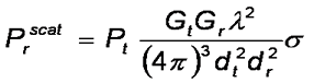
Rain Attenuation

The attenuation due to rain can be calculated from the ratio of the power flux in to the power flux out:

Which we can write as P(r) = P(0) e ^-αr, where α is the reciprocal of the range where P drops by 1/e. Writing this in dB form gives us:

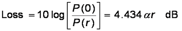
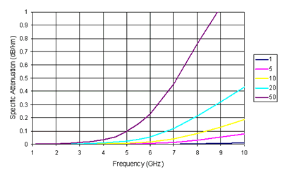
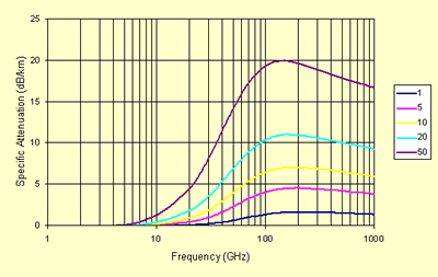
The value 4.343α is called the specific attenuation, γ which is usually expressed in dB/km. It can be calculated from EM theory if the drop size and shape distributions are known, but it is easier to take the standard model based on the rainfall rate:

Where a and b are constants provided in tables like the one below.

Note how a increases with frequency while b varies less, rain attenuation is much higher at high frequencies.

 

The total rain attenuation can be evaluated by integrating the specific attenuation along the path. In order to do this, all we need to know is how heavily it is raining at each point along the path. This information can be found from rain radar maps, or we can look up the statistics or rain rate and distribution for the part of the world we are located in.

 

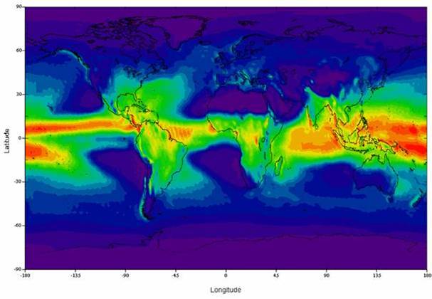
0.01% annual rainfall exceedance rate (Source ITU-R)

Rain is not particularly uniformly distributed, so a longer path the rainfall rate may vary quite a bit along the path. When working out rain fade margins, it is important to remember this and there are well defined methods, one of which is described in the systems section of this tutorial.

 

Rainscatter

We have already discussed the scattering of radiowaves by irregularities within the troposphere. Another effect that is particularly important above 3GHz is Rainscatter - or more strictly Hydrometeor scatter. Rainscatter can extend the propagation of microwave signals to well beyond line of sight. With scattering from rain at 2-4km above the ground, the range extension can be by several hundred km. A site that estimates rain scatter for amateur radio purposes based on weather radar is currently available at http://www.frontiernet.net/~aflowers/rainscatter/ .

 

Why Rain Scatters Radiowaves

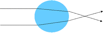
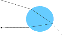
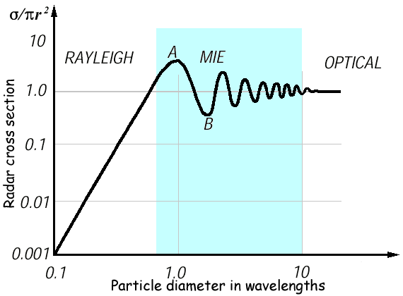
The forward scatter by Hydrometeors at microwaves is via a mechanism called Rayleigh scattering. Rayleigh wrote a paper about it in 1871, hence the name. Rayleigh type scattering occurs when the particle is electrically small and phase shift across the particle is small, that is the particle is much smaller than the wavelength. Rayleigh scattering scatters energy with a radiation pattern like that of a dipole, the amount of scattered energy is proportional to D³/λ. If the particle is of the order of the size of the wavelength, Mie scattering occurs. With Mie scattering, there is more forward scattering and a forward radiation lobe.

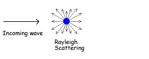
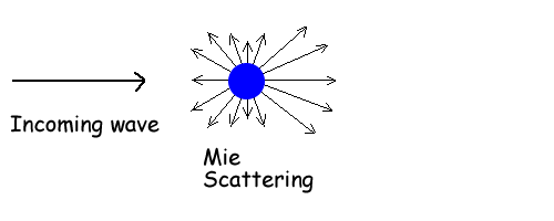
The Rayleigh and Mie are not different mechanisms, they are simply models approximating the scattering mechanism applicable at different wavelengths. The following diagram from a radar discussion demonstrates this well.

Scattering does not just affect radiowaves, scattering of light by molecules in the air is why the sky is not black. There is a wavelength dependence shorter wavelengths are scattered more than longer ones.

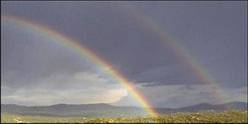
A practical example is the very small particles in the upper atmosphere scatter blue light more than red light because blue light has a shorter wavelength, hence the sky is blue. The very small water particles in clouds are still much larger than the wavelength of light, so there is no frequency selectivity and the scattered light is white. Large raindrops allow light to be internally reflected, with the refracted angle dependent on wavelength, hence the rainbow. Rainbows are colourful as red light which has the longer wavelength is refracted slightly less than blue light with the shorter wavelength.

This wavelength dependence is also why VHF and UHF signals are not significantly scattered whereas SHF and up signals are. Most of the scattering from rain for microwave signals can be considered to be Rayleigh scattering. The Rayleigh criterion:

πD/l <<1 where D is the diameter of the particle and

πnD/l <<1 where n is the refractive index.

If the above are true, the Rayleigh approximation can be made. A typical raindrop may have a diameter of 1mm so assuming a refractive index of 1 (see later) pnD/l = 1 if l ~ 3mm equivalent to around 100GHz. So for this 1mm raindrop if the frequency is below 100GHz we will observe Rayleigh scattering and scattered electrical field will be like that of a dipole.

 

Essential Features of Rain Scatter

Naturally being weather dependent, values vary considerably with time and space - so actually calculating the rainscatter from first principles signal requires complex integration, assuming the structure of the rain is known or can be modeled and will generally require a numerical integration using a computer programme. However the important features are:

that the received signal strength is proportional to:

• transmitted power (obviously)
• the common volume (this is the antenna beam intersection),
• the particle density (for example how hard it is raining)
• the scattering function So² (how well the particles scatter - for example how large they are, D⁶)

and is inversely proportional to:

• the 4th power of range
• the 4th power of the wavelength.

Of course, the rain also attenuates the energy in the radiowave, so the scattered power at the receiver will be reduced.

 

Simplified rainscatter model

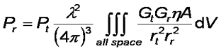
A simple model for bistatic rainscatter is shown below, it makes many assumptions to avoid any of the nasty maths - to do it properly we need to solve the equation:

This does not look too bad until you realise the functions of G, η and A are are fairly complex. To make it tractable we assume rain is a uniform cylinder as shown at the start of this section. The scattering volume then simplifies to the volume of a cylinder, which we know as:

Remembering h_r is around 3km and d_r ~ 3.3R^-0.08. for Heavy rain, R = 50mm/hr or more, d_r = 2.4km, V = 23 km³.

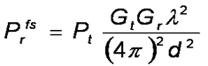
To calculate the scattered power we need to apply the bistatic radar equation. The power received by scatter from rain located at a distance d_r from the receiver is related to the power transmitted P_t at a distance d_t from the rain by:

Where σ is the scattering function we need to apply. A useful model for σ is:

S accounts for non-Rayleigh scatter, it is zero below 10 GHz. Above 10 GHz 10log S = R^0.4 4x10^-3 (f - 10)^1.6

S calculated for selected frequency bands

To use this equation, we need to know the common volume, which requires working out the intersection of the two antennas. A simple assumption to make is that the whole rain cell is within the common volume. This is not quite right, but is a good starting point if the path is long and the antennas beams are not too narrow. It is likely that we will overestimate a bit as frequently only the top of the rain cell will be visible to both antennas because of terrain blockage.

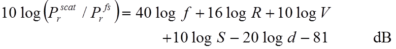
If we substitute the free space loss equation...

...into the bistatic radar equation

we can calculate a relative loss, which in dB:

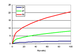
If you apply this model, which is simple enough in MsExcel you will get a plot like this for a 100km path, assuming the rain cell is at the mid point:

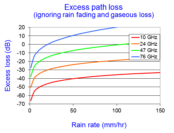
This is of course very wrong on several counts. Firstly, we can not get out ore energy than we put in and gains at the higher frequencies are unrelaistic. They arise as the model breaks down outside its intended range. In addition we can not get away from the presence of rain attenuation within the cell. Correcting for this requires yet another assumption, that the rain loss is only coming from this rain cell and that the average path length through rain for the scattered signal is equal to the diameter of the cell and that we can use the standard γ = a R^b formula. The result is shown below:

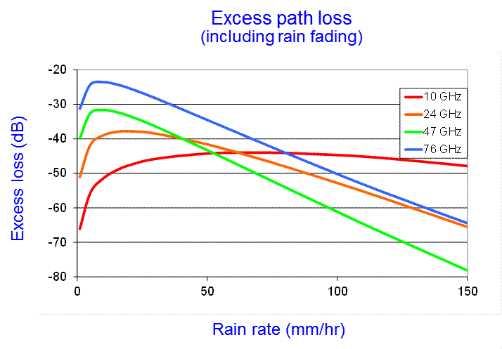
This is closer to what would be found in practice but be aware that this is a very simple model and the values though representative, can not be guaranteed, your mileage may vary, no responsibility will be accepted for losses caused by errors etc. etc..

Below 10 GHz rainscatter is still present, but quickly becomes less and less important as a propagation mechanism when compared to Troposcatter except for in very heavy rain.

Depolarisation

The non-spherical raindrop has another effect, depolarisation
Small rain drops are spherical but for diameters above 4mm, the base becomes concave.

Drop Size (mm)	2	4	6	Raindrop shape	Raindrop orientation
Axial ratio	0.92	0.82	0.65

Therefore different polarisations will propagate at different speeds through air containing rain and this will lead to differential phase shifts. They will also experience differential attenuation. Below 15 GHz most of the depolarisation comes from the differential phase shift and above 15 GHz most of the depolarisation comes from the differential attenuation.

If the polarisation plane (E-Field Vector) coincides with the symmetry of the raindrop, not a lot will change apart from the Horizontally polarised signal will be delayed relative to the vertical signal. If the drop is not aligned with the polarisation, for example if the drop is rotated by winds or if the polarisation is slanted or circular, energy will be transferred between the polarisation states. It is a good assumption for rain to assume the symmetry planes are close to vertical and horizontal, so H & V ploarised signals will not be depolarised by very much but slant polarised and circular polarised signals may be.

Definition of Cross Polar Discrimination (XPD) and Cross Polar Isolation (XPI)

Best done with a diagram.

  

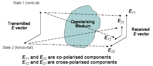
For rain, XPD and XPI are practically the same.

Depolarisation model

XPD is important if cross polar channels are used to increase capacity (e.g. satellite TV), this model works well to a first order

Where:

Sleet and Snow

The refractive index of water has a strong temperature dependence. The loss of ice is much less than that of water at Radio frequencies, the imaginary component of the refractive index of ice is low and consequently Ice is fairly lossless. Clouds, which contain ice crystals become important for mm-wave satellite links. Although fairly lossless, Needles of ice in clouds can cause large differential phase shifts and hence may degrade the XPD. Sleet consists of wet snow flakes which effectively look like very large raindrops. As a result, sleet can cause very high losses.

As ice absorption is very low the main loss mechanism for ice is scattering, which can also enhance signals beyond the horizon. Below ~100GHz a Rayleigh model can be used as for rain attenuation and rain scatter. Above 100 GHz we need to account for both Rayleigh and Mie scattering.

Frequency (GHz)	A (Mie) dB per km per g/m3	A (Rayleigh) dB per km per g/m3
300	15	15
400	20.5	20.3
500	26	25
800	41	38
1000	50	43

 

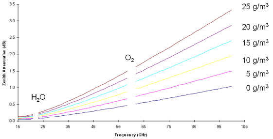
Clouds

Clouds cause significant loss on high frequency satellite links, the typical attenuation at Zenith (looking straight up) for cloudy sky is shown in the figure. While there is attenuation, it is only a few dB below 100 GHz.

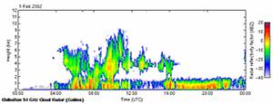
At the base of clouds a melting layer forms where, ice particles melt and become rain, this is a fairly turbulent region containing a mixture of rain, ice and snow. There is lots of scatter and loss, this is called the “Bright band” by the weather radar community. Propagation horizontally through it at high frequencies is bad news. This can happen in colder regions in the winter when the melting layer is relatively near the ground and microwave links from hilltops are in or above the melting layer.

Next