Fading Channels

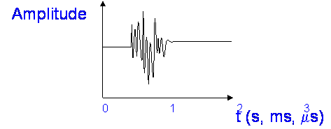
The signal amplitude at the receiver varies over time, we generally call this signal fading. We split this into slow fading and fast fading. Everything is relative, but this generally means variations in amplitude that change slowly with time. E.g slowly compared to the transmission frame length. Often engineers think of slow fading as being fading where the system might have time to react in some way, for example using an AGC system. Fast fading is signal variation that is considered too rapid for the system to follow.

Rain fading is an example of slow fading – with time variability measured in seconds and minutes. Mobile operators tend to consider shadowing by buildings as slow fading, periods of seconds while passing buildings.

Fast fading generally means variations in the signal amplitude that change rapidly with time, E.g. times of the order of a packet, or even a symbol.

Fast fading typically varies about a mean value and often fast fading is superimposed on slow fading. Multipath can cause fast fading in mobile systems. Tropospheric scintillation is another example of fast fading, though it is really a form of multipath too.

Models for fading channels

Firstly, consider the channel to be narrow band, that is the fading is flat across the channel bandwidth with no frequency selective fading. We can model flat fading channels as below:

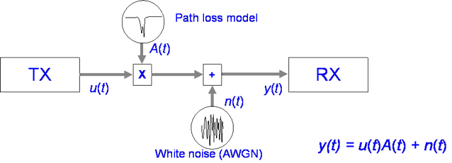
Often we combine two path loss models: one for slow variations, slow fading A(t) and another for fast variations, fast fading α(t)

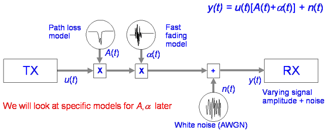
These models work well for channels that are not frequency selective, some narrow band fixed links for example, but they are not sufficient where there is frequency selective fading. We call such channels wideband channels and “Wideband” could mean 1GHz or 100Hz, it depends on the channel not the bandwidth compared to the centre frequency.

Wideband Channels

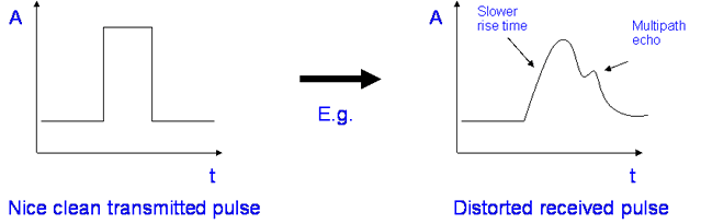
Ideally, we expect a channel to have a perfectly flat and linear frequency response. Frequently want to know the channel impulse response as we are interested in transmitting data.

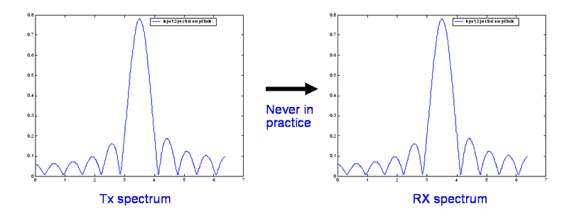
Real channels show distortion and the time domain representation is frequently used. The received pulse is distorted (always) because of the frequency and delay response of the channel.

 

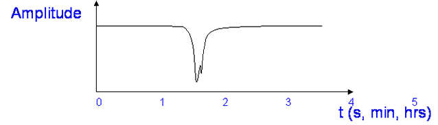
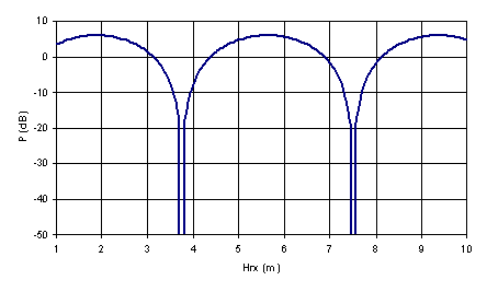
Multipath components are frequently present in mobile systems and if two components are of similar amplitude, they will interfere constructively and destructively as we have already seen in our ground reflection example:

If there is no energy in the channel, the receiver can not work – there are ways to overcome this, systems like OFDM used in Digital Terrestrial Television (DTT). Apart from this filtering effect – pulses are also spread out over time. We represent this with the channel impulse response:

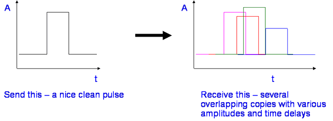
Typically, the receiver can not distinguish the resulting mess, unless it is specifically designed to (Rake, MIMO).

We define the number of components and delay parameters by applying a threshold which is often set so that 90% of the energy is contained. This is the “Delay Window”.

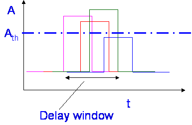
The number of components is the number in the delay window, the Delay Spread is a measure of the variability of the width of the delay window.

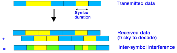
Importance of multipath delays

Data is traditionally transmitted in the time domain as a sequence of symbols. Each symbol has a set duration, for example at 1 Mbaud, each symbol lasts 1 µS.

Delay spread causes the error rate to cease to decrease with increased SNR. There is an error floor effect where increasing the power will not improve the error rate.

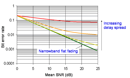
All digital systems have an error floor - but generally it helps if it is at a low error rate, like 10^-12 or better. By using coding techniques, it is possible to compensate for high channel error rates, though possibly not for a situation as bas as in the top line above.

The tapped delay line model

This is a popular model for multipath simulation work. We can model multipath a a series of amplitude weighted delayed copies of the input signal.

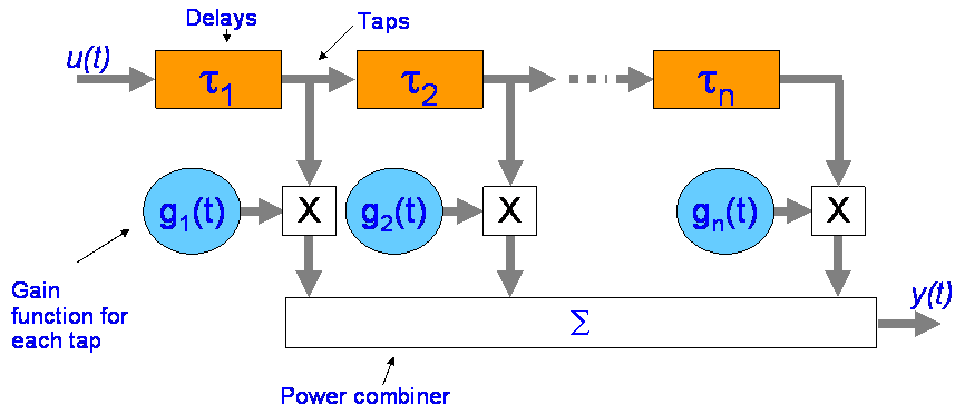
Note the taps considered uncorrelated. The delays &tau₁, &tau₂ … &tau_n are not fixed, but functions conforming to the delay spread.

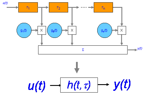
We define the impulse response h(t,τ) - the delay spread function

Defining Delay Spread

Here are a set of definitions for come common paramaters used in modeling multipath.

 

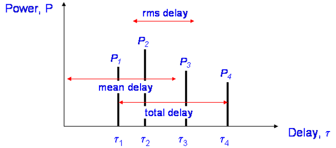
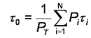
The received signal, P(t) made up from N taps P1(t) to PN (t)

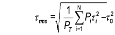
The rms delay spread is often quoted for various environments. Modern demodulators are able to de-spread and make use of the multipath components in the incoming signal and therefore gain a significant increase in signal energy. RAKE receivers are an example of this technology.

Delay spread Examples

Here are some typical values at 1-2 GHz for mobile systems. Inter-symbol interference occurs when the delay spread is similar to the symbol duration. For reference, one GSM symbol is 3.7µs long, so we worry about it most in Urban and Hilly areas.

Environment	rms delay spread (µS)
Indoor	0.01-0.05
Mobile satellite	0.04-0.05
Open area	< 0.2
Suburban macrocell	< 1
Urban macrocell	1-3
Hilly area macrocell	3-10

Frequency Domain

Not only are signals dispersed in time but also in frequency, Otherwise delays would be constant. It is just as valid to work in the frequency domain which leads to the phenomena of Doppler spread. This requires the transmitter, the receiver or the scattering object to be moving, the term “mobile radio” gives us a clue here…. It can also be caused by the medium moving or evolving, the Ionosphere for example.

There is another version of transfer function which is a filter with a time variant frequency response. It is called the Time Variant Transfer TVT function. This is actually the Fourier Transform of the delay spread function h(t,τ;)

 

Bello Functions

The relationships for the family of channel functions are named after a chap called Bello who defined them in 1963.

 

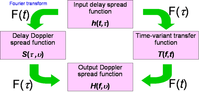
The Fourier transform and inverse Fourier transform is beyond the scope of this course, however it is useful to know that this is a model that allows us to move between the time domain and the frequency domain which can be easily implemented in DSP hardware.

Next