Diffraction

Diffraction is the "Bending” of wavefronts around obstacles. Diffraction occurs with all propagating waves, including sound waves, waves on water waves in materials and  electromagnetic waves. Diffraction always occurs, its effects are generally only noticeable for waves where the wavelength similar to the size of the diffracting object.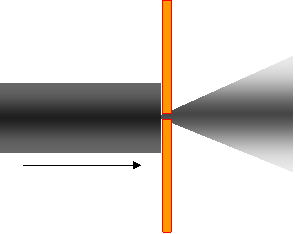

E.g. a Signal passing through a window

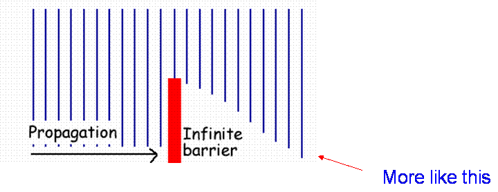
Diffraction is a large subject with some fairly difficult mathematics - we will try to limit the maths. What happens when an EM wave encounters a barrier?

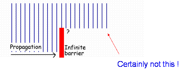
Signals diffract around the barrier

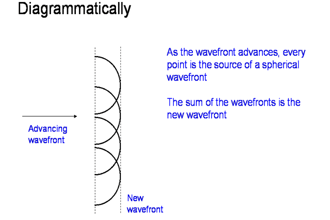
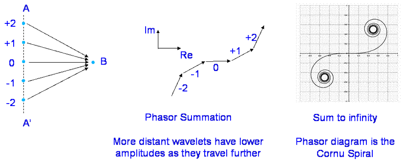
The Huygens construction

Christiaan Huygens (1629–1695) was a Dutch mathematician, astronomer and physicist. He came up with a theory that light was a wave. His rule is “Each point on a wavefront acts as a source of secondary wavelets. The combination of these secondary wavelets produces the new wavefront in the direction of propagation”.

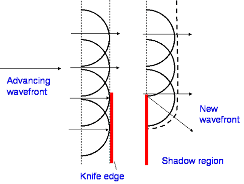
Diffraction over a perfectly absorbing knife edge can be understood through using Huygens construction:

 

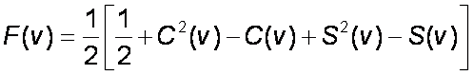
The Cornu spiral is developed from Huygens, summing the amplitude and phase of each wavelet. To find the field at B from the wavefront A-A’
Sum the wavelets -2,-1,0,1,2 accounting for vector nature of the field.

Now move a knife edge upwards and it cuts out the lower wavelets, effectively cutting out the lower part of the spiral

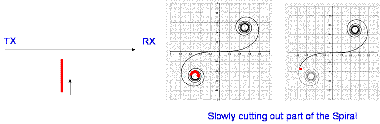
The effect of this is initially an oscillation then as the direct path is cut off, a signal loss.

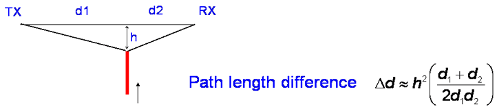
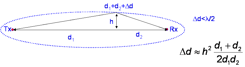
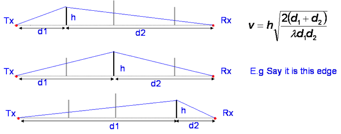
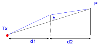
Estimating the diffraction loss

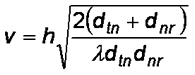
Consider this geometry of a Knife edge gradually cutting off the wavefront. Also h << d1, d2 and λ<< d1,d2

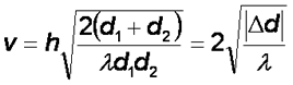
Define parameter v:

Be careful with the sign if you use this last one, v is negative when edge is below the direct path.

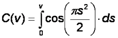
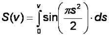
The Cornu spiral is given to a good approximation by plotting the Fresnel Sine and Cosine integrals of v, where:

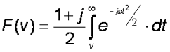
The E field can be expressed by summing from the top of the knife edge to infinity.

..Which is beyond this tutorial…but can be written as:

Which we could work out but fortunately there is a very good approximation:

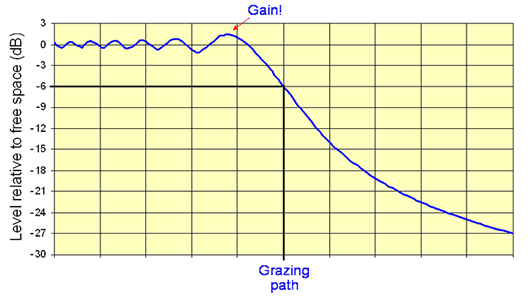
Here it is plotted:

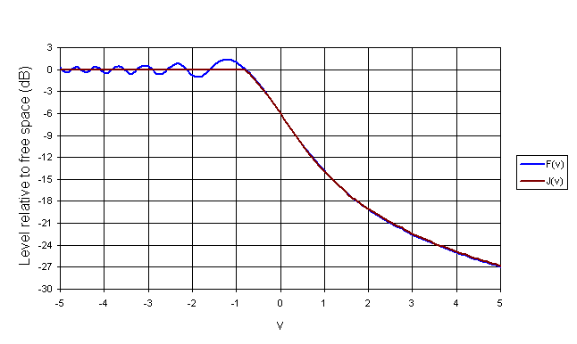
Note: For a grazing knife edge, h = 0 so v = 0, giving a 6 dB loss. For first Fresnel zone clearance, v < -1.4, no loss).

 

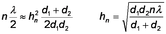
Fresnel zones

I have mentioned these several times so I had better define them. From diffraction theory, it is clear that the effect of the knife edge begins before the direct path is cut. Some clearance is needed and the amount is expressed in terms of Fresnel zones. The first Fresnel zone is the locus of points where the additional path length compared with the shortest path does not exceed λ/2.

Further Fresnel zones are defined by additional 1/2 wavelength path length increments.

 

 

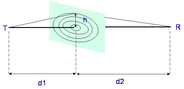
Line of Sight?

We generally assume line of sight clearance if more than 0.6 of the 1st Fresnel zone diameter is cleared.

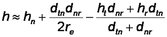
Calculating Knife edge losses over the Earth

It is necessary to account for the curvature of the earth and for any slope in the path to calculate how far a knife edge impinges on a path. We do this by defining everything relative to a reference plane.

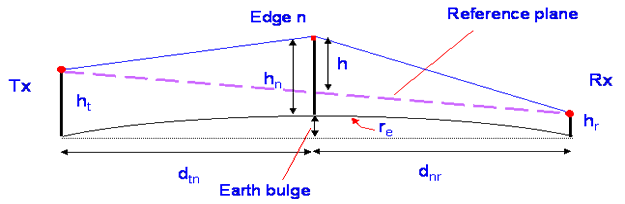
As long as the path length is much greater than the height of the obstacle, which it usually is, we can make an approximation for the height of the edge above the reference plane. It is this height that is used in the diffraction calculation.

So the diffraction parameter v is given by:

Which can be used to calculate the path loss from the equation for J(v)

 

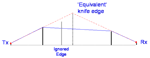
Multiple Edges

What should we do if there is more than one obstruction? There are several models commonly used, including those by Bullington, Epstein-Petersen, Deygout, etc. They are all approximations and have potential for errors, especially with closely spaced edges. They differ in how they calculate the geometry and hence the parameter v and they differ in how many edges they take into account and how they add up the loses.

Bullington

The Bullington method is quite simple, it is based on constructing an equivalent single knife edge at the intersection of Tx/Rx “horizons” and calculating the loss based on that. It is easy to do but is prone to underestimate loss as it can ignore important intermediate edges.

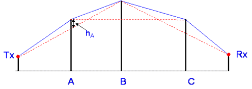
Epstein-Peterson

Sums up the loss for each single edge in turn, using height above dotted line as the effective height of edge. Potentially a better method but causes large errors on paths with closely spaced edges.

Deygout(the principle edge method)

This method is more involved, it splits the path into segments. Firstly we need to find edge with largest value of parameter v, ignoring all other edges. This is called the “Principle Edge” and its v parameter is saved.

Now working from the principle edge P, we treat as if there is a new path between the TX and the principle edge and create a new reference plane and calculate v for the intermediate edge, if there is one, based on the height above the reference plane.

This edge will have a lower value of v and becomes the principle edge for the path from Tx to P. The process is recursive for multiple intermediate edges and can be repeated until all edges are considered. The method ignore any edges with 1st Fresnel zone clearance. The same process is used along the path from P to the receiver.

At the end of the procedure we will have a set of J(v) losses for each edge - the method simply adds these up. So for 3 edges:

Generally, modified Deygout methods are used with fudge factors and scaling factors to further improve the accuracy compared to measurements.

Real Terrain

Normal terrain, hills etc do not really look like knife edges and is often better represented by cylinders, which have a higher loss.

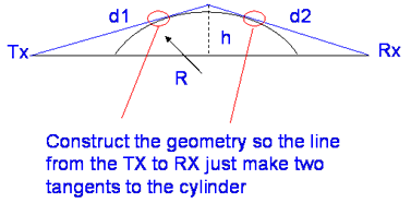
Fortunately, we can approximate the additional loss, L = J(v) + T where T is an additional loss that accounts for diffraction at the tangents to the cylinder.

Most real-world obstructions are not like knife edges and it is only possible to solve the equations for idealised cases. Solutions for many objects and including reflection effects, loss from trees etc. rapidly become impractical and in many cases. Usually we do not really know enough detail about the exact nature of the terrain anyway. For example mobile systems would need re-analysing every 0.1 wavelengths and for 3G systems that would require a terrain map with points every 1.5cm. To overcome this and make a best guess, path loss prediction models are used, we will come on to these later.

Next