Link Budgets

In the following sections of the tutorial we will change emphasis a bit and start to look in particular at the effects of radiowave propagation on channels. We will cover link budgets, noise, wide band effects, modeling and measurement techniques.

Link Budgets

This is all about finding the signal level received from the signal level transmitted. A link budget is a formal way of calculating the expected received signal to noise ratio. This is something designers generally want to know to make design decisions like what antenna gain and how much transmitter power is needed. This effects the hardware cost and is important in satisfying the license conditions etc. Knowing how to properly make a link budget is a very important skill for a communications system design engineer. Some people make a lot of money out of being able to do it well. It is at the basis of antennas and propagation studies as the path loss between the terminals depends only on the propagation loss and the antenna gain.

Link budgets usually start with the transmitter power and sum all the gains and losses in the system accounting for the propagation losses to find the received power. Then the noise level at the receiver is estimated so we can take the ratio of the signal power to the noise power and work out the performance of the link. This procedure is shown for the generic system below:

The 3 steps are

What is not included yet in the above in order to avoid confusion is the interference. Interference can often be treated like additional noise, but the effect of interference depends very much on the modulation scheme being used. With digital systems, interference can be treated as noise, but beware of pulse type interference, which may have a low average power but can completely disrupt services like DTT and DAB through causing bursts of unrecoverable errors that prevent the highly compressed content from being decoded.

EIRP

The transmitter parameters are often further simplified using the concept of EIRP. This is useful as it allows us to treat systems with very different antenna characteristics similarly.

In radio systems, the Equivalent Isotropically Radiated Power (EIRP) is the amount of power that would have to be radiated by an isotropic antenna to produce the equivalent power density observed from the actual antenna in a specified direction. The EIRP is still a function of direction, we are not assuming power is radiated isotropically. Usually EIRP is quoted for bore sight, defined as the axis of maximum radiation. Occasionally we need to refer to the off axis EIRP which may be in the direction of another system that is suffering interference.

The EIRP is usually quoted in decibels compared to a reference power, e.g. 1watt,  0dBW or 1 milliwatt 0dBm. The EIRP is a useful quantity for comparing systems as it is system independent, that is we do not need to know anything else in order to calculate the radiated field strength.

Path Losses

We now need to consider the link parameters - the path loss, which we know this already, it is the sum of all the losses between transmitter and receiver that are not to do with the antennas or feeders.

Path loss = Free space loss + Gas loss + Additional path loss

Signal power at receiver

We now have enough information to calculate the signal power at the receiver:

Received power = EIRP - Path Loss + Receiver antenna gain

E.g. Handheld radio 448 MHz, EIRP ~ 0.5 Watt = -3 dBW, Antenna gain, 0 dB (Isotropic) so for a 1km line of sight path, the loss = 85 dB and the received power = -88 dBW (That is a strong signal). It is easy, but we have assumed the receiver is linear. With high received signal powers from -40 dBW upwards, this becomes less likely. Many strong signals at a receiver may cause undesirable intermodulation products to be generated which will degrade the performance.

Noise power at the receiver

We are half way to finishing our link budget with the signal power at the receiver. We need to know the noise power to find the signal to noise ratio. Noise comes from several sources, there is natural noise from the environment, noise generated within the receiver itself and man made noise. Everything with a temperature will generate noise - Boltzmann’s law says the noise power per unit bandwidth = kT where k is Boltzmann’s constant and T is the absolute temperature in Kelvin.

Important features of this type of noise is that noise is additive, if you have two noise sources you get the sum of the noise power from each, and noise has a flat spectrum, so if you increase the bandwidth you increase the noise power in proportion.

Boltzmann’s constant is often expressed in the units of dB Watts per Hz per Kelvin, that is how many watts you get per Hz of bandwidth for each Kelvin of temperature. Its value is -228.6 dBw/HzK. For example you might an antenna looking at the ground has a noise temperature of 290K. The noise power received in a 1MHz bandwidth at a noise temperature of 290K is:

                                  Noise power per MHz =   -228.6 + 60 + 24.6 = -144 dBW

Some typical values are shown in the figure:

There is some evidence that the man made noise levels are increasing in some environments. This is a hot topic as Ultra-Wideband systems intend to operate below the noise floor of conventional systems and there is some disagreement between the UWB and conventional camps over what that level is.

Another issue is over power line transmission PLT technology, which used mains wiring to send data in the vein hope that the wires will not radiate. They do radiate of course and the aim is to keep the additional noise to below the current noise floor – this dispute is quite heated because prototype PLT systems have been demonstrated by the BBC to be severely damaging to broadcast reception.

Noise at the antenna

The antenna picks up noise from the sources in the previous slide, depending on its radiation pattern, it also generates noise through its own temperature and losses and picks up noise from the Earth at 290K in the sidelobes. To estimate the noise picked up by an antenna, a quick method is to take the antenna efficiency as an indication of the sidelobe power. So, if the efficiency is 60%, the external noise in the direction of the antenna accounts for 60% and the sidelobes represent 40% of the noise pickup. It is further assumed that half of the sidelobes are looking towards the sky and half towards the ground. For example, with a 60% efficient dish as might be used for satellite TV reception at 12GHz, the sky noise temperature may be ~15K and the ground noise temperature 200K. The total antenna noise is estimated as:

                                Antenna noise temperature = 0.6 x 15K + 0.4 x (15K + 200K)/2 = 52K

The ratio is nearly 4 times compared to what it would be without the sidelobes, so dish efficiency can sometimes matter even more for noise than it does for received signal power.

Noise generated in the receiver

Noise is generated by all inline devices, for example passive devices including attenuators, waveguides, cables, filters etc. or active devices, amplifiers, mixers etc. Each can be represented reasonably accurately as an additional noise source (resistor) at the input to the system:

Passive Devices

If a passive device has loss it will add noise to the system proportional to its temperature (Assumed 290K unless known) and the loss.

Nothing adds no noise unless it has a temperature of absolute zero. Feeders always have loss. The loss at microwave frequencies is higher and feeder lengths need to be minimised to obtain a low overall system noise temperature. Radio astronomy stations whose performance would be totally devastated by a 75K feeder temperature dispense with the feeder altogether. They use beam waveguides where the only loss is in the reflecting surfaces – which is low because of their size plus they can be easily cooled.

Active Devices

All active devices generate noise internally, the reasons are complex, but it can be modeled as an effective noise temperature, e.g. for an amplifier:

Typical noise temperatures for real amplifiers are in range 10K - 1000K. The Noise Factor is a measure of how much noise is added by an active device. When the receiver is matched by a load resistor at standard temperature T₀ 290K noise power input is:

Noise Factor F = (Noise Out / Noise In) – referenced to input!

Noise Factor:

Which if expressed in dB is F_dB = 10log(F) we call this the noise figure.

Alternatively, we can consider an Effective noise temperature:

and

Cascaded Sources

When a device is described as having a noise temperature or a noise figure, this is always relative to the INPUT of the device. When summing noise contributions we need to be careful about gain and loss, an amplifier will amplify input noise as well as the signal and a lossy device will attenuate input noise as well as adding noise due to its own noise temperature.

P_total = G₁G₂G₃...G_nkT₀B + G₁G₂G₃...G_nkT₁B + G₂G₃...G_nkT₃B + G₃...G_nkT_nB + …

Input x total gain     1st x total gain      2nd x (total gain – gain of 1st stage)...

This tells us something useful – if we have enough gain in our front end low noise amplifier, the noise figure of the rest of the receiver is of secondary importance. There is a trade off though as too much gain is bad for performance.  The problem is that putting gain at the front end of the receiver before the filtering reduces the systems immunity to strong out of band signals. Too much overall gain will add to the inter-modulation distortion generated from in-band signals and thereby reduce the dynamic range of the receiver.

Example

Find the overall noise figure of a receiver with a 10 dB noise figure preceded by an amplifier with a noise figure of 0.5 dB and a gain of 20 dB ?

To solve this we need to sum the input noise plus the noise temperature of the amplifier multiplied by the gain of the amplifier plus the noise temperature of the original receiver.

(Rearrange the equation P_total = G₁kT₀B + G₁kT₁B + kT₂B)

We have assumed a 60% antenna efficiency, that is quite a challenge for a mass market product. When satellite TV first became popular the original LNBs had noise temperatures of about 250K so the total noise temperature was 300K and the extra noise from the antenna really didn’t make that much difference. Nowadays LNBs are apparently available with noise temperatures of around 50K giving a total noise temperature of 100K. Now the antenna is responsible for half of the noise power. The LNB improvement equates to an improvement of 4.7 dB in SNR. That is more than enough gained to permit the dish size to be reduced to 45cm. An even smaller dish could be used if it was not for the congestion in the Geostationary orbit. Instead, we now use 45cm and the improvements in LNBs have allowed an increased data rate.

Why worry about noise figure?

Say we have a receiver with a noise figure of 10 dB and 20MHz bandwidth. What is the equivalent noise power?

The receiver noise floor is – 121 dBW. Say we are looking for a TV satellite, with a good antenna so the antenna noise temperature is low, maybe 50K, if we work out the input noise power we find it is:

So our receiver noise is much higher than the input noise, with at –121 dBW being 18 dB worse than it would be an ideal noiseless receiver. An input signal of –120 dBW from a transponder would have an SNR of 1 dB, if our system was noiseless this could have been 19 dB.

To fix this the manufacturer fits a 0.5 dB NF LNA , which as we know gave us 61K of additional noise, which when added to the antenna noise gives a a total of 111K.

The signal would now have an SNR of 15 dB! That is the difference between a good watchable picture and none at all. If we did not have the low noise amplifier the satellite operator would need to compensate with 14 dB more power, which would be economic suicide.

In perspective

Remember to keep noise temperatures in perspective, there is usually no need for one part of a system to have a vastly better noise performance than another. Low noise receivers are important in space and satellite systems but much less important for terrestrial systems in noisy environments.

In a typical business area, at UHF the noise temperature seen by the antenna will be 1000K or more. This is similar to T_e for our example so improving our 10 dB NF receiver is not going to make such a large difference to the signal to noise ratio. Adding a 20 dB gain amplifier in front would actually make the receiver worse as it would affect the strong signal handling – there lots of strong signals around in industrial areas.

Things are different for SETI trying to look for ET at π times the hydrogen line (~4.5 GHz) from a quiet location with a good antenna with input noise ~ 10K. Even the receiver noise temperature of 61K would be considered poor and Cryogenic cooling and very low noise systems are needed for radio astronomy.

Summary

Do link budgets in dB as it is easier. The steps are:
Find the Signal (dBW)

Find the Noise (dBW)

Find the SNR (dB) = Signal (dBW) – Noise (dBW)

Some Examples
Voyager - again. Last time we calculated Goldstone received a signal level of -180 dBW from Voyager. Building on our previous example, what is the data rate one might expect to be able to receive from a space probe.

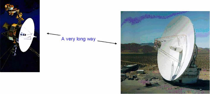
Goldstone uses the best LNAs available and the system noise temperature is around 30k. The antenna is designed for very low sidelobe noise
and it tends to not be used at low elevation angles. Goldstone uses cryogenic cooling on the LNAs, much of the noise power comes from the waveguide loss of 0.2 dB, equivalent to a noise temperature of 14K. The rest comes from the atmospheric loss and antenna noise temperature, both of which depend on the elevation angle. This equates to a noise power of:

The S/N is the difference:

Shannon's theory says in the limit we get no errors with a bit energy to noise energy ratio of -1.6 dB. Some modern exotic schemes get to within a dB or so of this, but remember Voyager was designed in the 1970s. The coding scheme deployed needs a bit energy to noise energy ratio of 2.5 dB which gives us a maximum data rate 33.8 – 2.5 = 31.3 dB/Hz, which is equivalent to 1.35 kb/s.

(note: we have ignored several degradations, for example Goldstone’s antenna efficiency, in this link budget to avoid clouding the point)

A PMR system

Back to our PMR448 - What is the maximum line of sight range?

Radio specification:

Handheld radio 448 MHz, TX ~ 0.5 Watt
Antenna gain, 0 dB (Isotropic)
Noise figure = 6 dB, Bandwidth = 25kHz
Minimum usable SNR 12 dB

Find the noise floor:

Transmitted Power (EIRP):

Maximum path loss capability:

This is simply the difference between the EIRP and the required power, so we need to find minimum required signal power:

We need 12 dB SNR to communicate so the signal power must be at least 12 dB above the noise floor

Required power = –155+12 = -143 dBW

Path loss capability = (-3) - (-143) = 140 dB

Path loss with distance:

At this frequency gases can be ignored, so the line of sight path loss is given by

This should equal 140 dB, so

The reason that PMR 448 handies don’t work over 537km because there are not usually any 537km line of sight paths. We have of course completely forgotten about interference here. Interference is frequently the major limiting factor in mobile communications systems. That is why it is important to understand the propagation characteristics of unwanted co-channel signals as well as wanted ones.

Next