
The Fundementals
Introduction Maxwell's equations Plane waves Free space loss Gas Loss Refraction Diffraction Reflections Troposcatter Rain effects Vegetation Statistics Link budgets Noise Multipath Measurements Models
Developing models
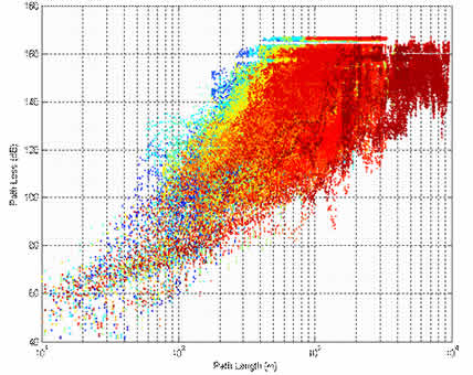
So you have some measurements, what can we do with them. Here is an example of path loss against range for some mobile drive around trials. There is a clear trend with distance but considerable spread. It is clear that distance is not the only important parameter. For mobile measurements, the effect of the clutter is likely to be significant and that is what is happening here.
Site General vs Site Specific
The following are not hard definitions. A statistical model can be made up by simulation using a specific model for many sites.
Site General Models
These models predict the distribution of effects over a population of terminals, they tend to be based on fits to large numbers of measurements. They frequently only need limited input data that is easy to obtain and while statistically accurate they are generalised over locations etc.
Site Specific Models
These are predictions for a specific situation or site. They may be based on fewer but more detailed measurements and tend to require more detailed input data than the general models, which may be expensive to collect.
Fits to data
With general models, be very wary of curve fitting
- especially where there may be measurement errors. It is always possible
to define a model that passes through all the measured data points, but there
is no guarantee it will not give serious errors at points where no data was
measured.
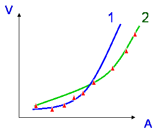
The blue model below is a perfect fit to data - but is possibly unlikely.
The green model is not such a good fit, but it is more likely to be true.
It is important to make sure there are enough parameters.
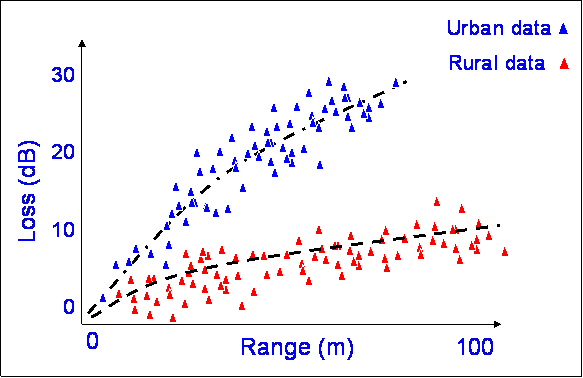
This often happens - there are two clear trends in the data, due to different propagation effects. A model based only on range would be poor. This type of multimodal data could be caused by there being a higher loss with distance in the urban area because of the effects of buildings. Similar plots can be shown for horizontal vs vertical polarisation through rain.
Input Parameters
It is obvious but the input parameters
must be available, they should capture the important features of the mechanism
but we do not want too many parameters. Too many parameters and options makes
it difficult to implement a model algorithm in a computer programme. It becomes
very difficult to test the stability and accuracy of the model when there
are very many parameters so parameters that have only a minor effect should
be neglected. Recent advances in computing power mean there is now much more
parametric data available that we can realistically deal with, storage capability
is large, computers are fast, so we have things like accurate models of buildings.
We can now model propagation in cities with good accuracy. Some examples of
input parameters:
| System | Frequency, bandwidth, polarisation, antenna pattern
|
| Path | Path length, location, path profile, height, elevation angle
|
| Climate | Temperature, pressure, humidity & lapse rates Rain rate, type of rain (stratiform, convective) incidence of fog, Seasonal variability of climate parameters |
| Environment | Urban, suburban, rural, forest, Building databases, building materials, vegetation type |
Model Testing
Generally, if there is a difference between the measurements and the model
– the measurements are right, but note there may be measurement errors. The
model error is defined as the difference between the measurement and the prediction.
![]()
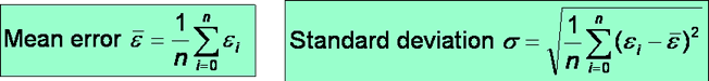
We tend to look for a mean error and a standard deviation from this mean:
Sometimes, we wish to weight the significance of errors according to the value
of the measurement. Which of models 1 or 2 is best depends on which end of
the curve you are interested in.
Often we don’t care so much if a model miss-predicts the 90% level as long as it gets the 99.9% value right - say we are interested in the predicting a maximum fade depth margin. Getting the 99.9% level right will automatically ensure there is enough margin for 90%. All this means that:
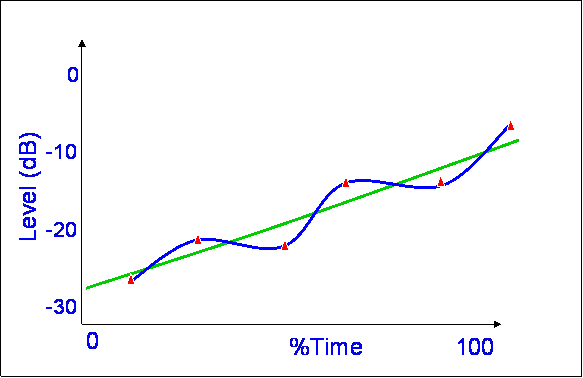
This results in the subject of Testing variables. In order to judge the relative merits of a prediction method, an objective set of criteria needs to be defined based on what we are interested in predicting which usually ends up being some test variable that should be minimised (or maximised). Here is one for rain attenuation from the ITU-R as an example:
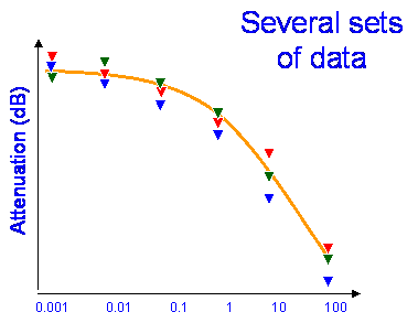 |
The picture shows a model for rain attenuation compared with some measured values of the percentage of time attenuation (A) will not be exceeded e.g.:
|
The ratio of the predicted and measured values at each percentage step from 0.001 to 100 are computed for each data series:
Where: i = link number, p = predicted, m = measured.
The test variable is found from:
Vi = ln Si (Am,i / 10)0.2 for Am,i < 10 dB = ln Si for Am,i ³ 10 dB
It is assumed in this model that the modulus of S is taken - don’t take logs
of negative numbers for this application. This operation creates a bias against
low attenuations. Next calculate the mean (µv) and SD (σv)
of the Vi values for each percentage of time.
Then find the testing variable ρv from:
The value of ρv should be minimised.
This test variable has caused some debate. The intention is to bias the model
testing to those that correctly predict the higher levels of attenuation.
This is useful as there is often measurement uncertainty that can give high
relative errors that are not really very important - e.g. 1dB to 2 dB is a
ratio of 2 but only 1 dB but 10 dB to 20dB is the same ratio but rather more
significant.
© Mike Willis May 5th, 2007
