Measurements

Measurements are needed for developing propagation models and models are needed for design and planning. Developing models from Maxwell’s equations is often not practical We don’t always have enough environmental data for a completely deterministic solution. The type of measurement required depends on the service. Long term statistics measured over many years are needed to assess fading distributions on microwave links. Here we are interested in events that only last for a few minutes per year, so for example 0.01% of a year is only 53 minutes, and it takes many years to get a reliable measurement. A large number of short term measurements are needed to test a mobile coverage prediction model. Here we are more interested in probabilities of call failure of a few percent but for a very large number of locations.

Beacon measurements are typically used in satcoms and terrestrial links when a long term measurement is needed. A reliable test signal (usually CW) is sent and this is received and recorded by a beacon receiver, made up from specialised hardware designed to give accurate long term results. A large dynamic range often needed and the system must be very stable over a long time which means it will be probably be expensive. There are many years of measurements available in ITU-R databases etc.

Here is an example of a long term measurement, in this case the beacons on the Olympus satellite, which was at an elevation of around 30⁰.

The monthly statistics for 30 GHz below show that there is considerable monthly variability. This tells us we will need many months of measurement to get a good idea of the “average”. Note the similar curve shapes - this implies the “worst month” can be found by scaling from the average value.

Drive round measurements are commonly used for mobile systems. A transmitter is set up in a “typical” location to represent a base station and a measurement vehicle drives a set route. GPS etc. is used for positioning and databases and aerial photos used for analysis.

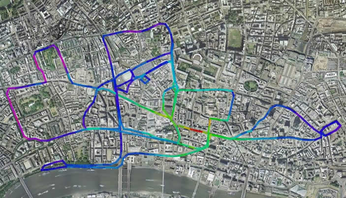
Google Earth now has some very useful mapping and visualisation tools built in. The image above was produced by submitting a track file of lat, long and signal strength to the software. It is then possible to zoom in and around the track and note the effects of the street layout on the received signal level.

What to measure

Measuring power might not be sufficient, there could be Doppler spreading, delay spread e.g. rain scatter. To measure these we often use channel sounders. There are many types, put “Channel sounder” into Google and you will get hundreds of hits, it is a big business. One method is to transmit a known pseudo random sequence and at the receiver use a sliding correlator to resolve individual multipath components. A very simple sounder is shown diagramatically below:

In this type of sounder the resolution and ambiguity depend on the length and rate of the PN sequence.

Channel Sensing

More advanced communications systems sense the channel to make optimum use of it. Most modern cell phones do this. This can be an active negotiation between transmitter and receiver, or it can be only at the receiver, the latter is necessary for broadcast. A sophisticated scheme is used in the new standard for digital HF broadcasting, DRM. HF links via ionospheric reflection can suffer severe delay and Doppler spreading.

The DREAM software package is an open source DRM decoder based on DSP. It is shown here receiving RTL at ~6 MHz at a data rate 21kb/s in 10kHz, mode B. DRM mode B in 10kHz uses 206 COFDM carriers and here they are modulated with 64QAM. The dialogue is telling us we have an SNR of 21.6 dB and a delay spread of 3.59mS. A symbol in this transmission mode lasts 27mS so this is not a problem - the signal decodes properly.

 

The software can measure the channel impulse response, here the decoder has used known patterns the received signal to measure the channel impulse response - the DRM standard includes special symbols to aid channel estimation.

The plots are a few seconds apart and four components are detected. Note the delay spacing is ~2mS (600km), probably an F-layer reflection 300km up. This is the resulting DRM superframe of about 1.2 seconds at the decision stage:

There are many samples of each of the 206 carriers superimposed in this constallation - but you can make out the FAC codes and SDC codes which are designed to aid data recovery and identify the transmission. The FACs are 3 dedicated pilot carriers transmitted at offsets of 750 Hz, 2250 Hz, 3000 Hz that always use QPSK modulation so they may be more robustly decoded. Their power is usually double that of the other carriers to help frequency acquisition. They contain 64 bits of data plus 8 bits parity that tell the decoder the transmission mode and what the multiplex contains.

The SDC is a service descriptor and it is only sent at the beginning of each transmission frame. It contains useful information like the station name and programme schedules.

Next