
The Fundementals
Introduction Maxwell's equations Plane waves Free space loss Gas Loss Refraction Diffraction Reflections Troposcatter Rain effects Vegetation Statistics Link budgets Noise Multipath Measurements Models
Signals and Noise
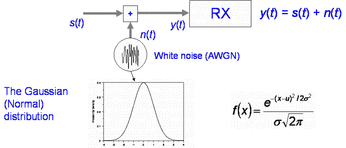
An exact copy of the signal transmitted is not what is received at the receiver. Noise is added to the signal, the amplitude and phase of the signal varies with time and location, there is a time delay which may be variable and the signal shape is distorted. So far we have treated noise as a purely random signal which is added at the receiver input, we call this Additive White Gaussian Noise (AWGN).

I and Q representation
Typically, we represent signals as their complex
baseband equivalents, I and Q representation where I and Q are orthogonal
and represented as a complex number:
n(t) = xn(t) + jyn(t)
Where x and y are random variables of zero mean. The mean noise power is related to the noise variance.
We will almost always treat noise as additive and Gaussian.
Showing ![]()
We know we can represent a random variable by its Probability Density function p(x). The probability the value lies between two values a and b is:
So the probability a value is less than a is:
We call P the cumulative distribution and so also the area between a and
b is the probability below b minus probability below a;
The Expectation of some function f(x) of a random variable x is:
Expectation is a statistical term referring to the
Expected (average) value of the function. Here we are interested in the Expectation
(mean) of x,
which we get if we set f(x) = x. This is often called the first moment of
x in statistics.
The variance is given by:
To find the power of complex signal n(t) we multiply by the complex conjugate.
The mean power is the expectation of N(t):
Expectation is a statistical term, according to Wikipedia:
In probability theory the expected value (or mathematical expectation) of a random variable is the sum of the probability of each possible outcome of the experiment multiplied by its payoff ("value"). Thus, it represents the average amount one "expects" as the outcome of the random trial when identical odds are repeated many times. Note that the value itself may not be expected in the general sense; it may be unlikely or even impossible. For example, the expected value from the roll of an ordinary six-sided die is 3.5, which is not one of the possible outcomes.
Remember that xn and yn oscillate about zero, which means their mean values are zero.
so
© Mike Willis May 5th, 2007