
The Fundementals
Introduction Maxwell's equations Plane waves Free space loss Gas Loss Refraction Diffraction Reflections Troposcatter Rain effects Vegetation Statistics Link budgets Noise Multipath Measurements Models
Propagation in the Atmosphere
This section is mainly concerned with the effects of the Troposphere, the lowest region of the atmosphere that extends upwards to about 10-20km. We are interested in the effects of the air and the weather on radio wave propagation.
Structure of the Atmosphere
The figure below shows the layers of the atmosphere.
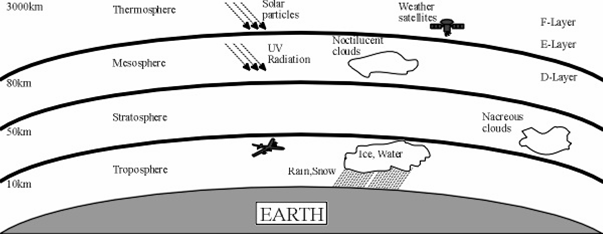
Moving upwards from the ground the layers which are differentiated by the variation of temperature with height are:
Troposphere: From the ground continuing up to between 7 km at the poles and 17 km at the equator with some variation due to weather. It is the thinnest but most dense layer, with 72% of the total mass of the atmosphere is below 10 000m. The troposphere is well mixed mixing due to solar heating at the surface. This heating warms air masses near the ground, which then rise as thermals. On average, temperature decreases with height.
Stratosphere: This extends from the top of the troposphere (7–17 km) up to around 50 km. In the stratosphere temperature increases with height.
Mesosphere: This extends from about 50 km to around 80-85 km. Temperature decreases with height.
Thermosphere: This extends from 80–85 km to in excess of 600km. The temperature increases with height. The Thermosphere is the boundary of the atmosphere, beyond the Thermosphere is the Exosphere, which extends into space.
The boundaries between the layers are the tropopause, the stratopause, the mesopause and the thermopause.
Gaseous Attenuation
A major difference in propagation through the atmosphere vs. free space is that there is air present. Air is made up of:
With Trace quantities of: Methane (CH4), Sulphur dioxide (SO2), Ozone (O3), Nitrogen oxide (NO) Nitrogen Dioxide (NO2). There are other gases too, as well as particulates and pollution.
Gas molecules interact with the radiowave electromagnetic field. This may cause energy loss E.g. H2O molecules are asymmetric and will try and align with the Electric field.
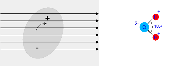
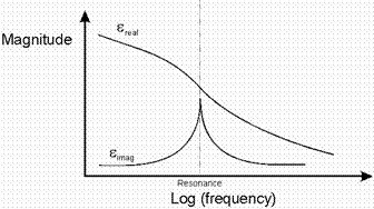
There are other interactions too, magnetic field interacting with molecular oscillations etc. Here is an example of a resonance line – the graph shows shows the real and imaginary parts of the permittivity versus frequency.
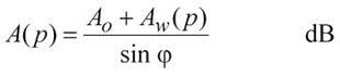
The amount of loss depends on the proximity to the resonant frequency - "absorption line" of the Gas molecules in question, the loss tangent of the resonance, the concentration of the Gas in the atmosphere and of course the length of the path through the gas. Atmospheric pressure also has an effect as it broadens the resonance lines through the collisions between molecules.The two gases that are most significant to radiowaves up to 300GHz are Water Vapour and Oxygen. The specific attenuation, (which is the attenuation for a 1km path), at sea level, due to Oxygen and water vapour is shown in the diagram below.
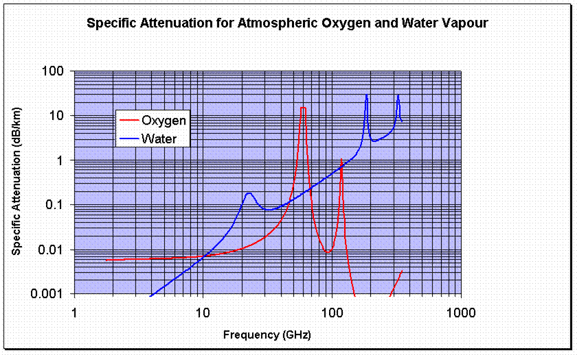
The resonance lines that are most significant up to 300GHz are those of water vapour at 22.3, 183.3 and 323.8 GHz and those of Oxygen where there is a series of lines between 57 and 63 GHz with another line at 118.74 GHz.
The specific attenuation at a given frequency can be calculated by summing the effects of all the significant resonance lines, this requires a computer programme. The ITU-R Recommendation P.676 contains several detailed models…..and there is a simple model too, a curve fit which we will look at next.
Rough & Ready Model for Sea Level Gaseous Attenuation
For water vapour attenuation, the model which is valid to 350 GHz is:
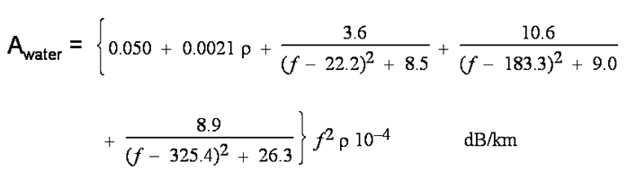
Where ρ is the water vapour concentration in
g/m3 and f is the frequency in GHz.
For Oxygen attenuation it is a bit more complicated with two models, one for frequencies below 57 GHz and one for above frequencies 63 GHz. For 57-63 GHz, an averaged value of 14.9 dB/km is used.


Where: f is the frequency in GHz.
The total combined attenuation is then found by
adding together the specific attenuation figures above. Given the specific
attenuation in dB/km, you can then calculate the total loss along a path by
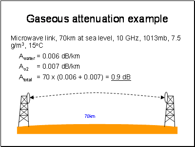
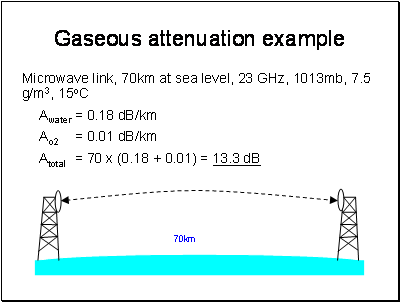
multiplying by the path length. A couple of examples:
Paths not at Sea Level?
This simple model relates to links at sea level. For higher altitudes, to a first approximation simply scale by the reduction in atmospheric density of the water vapour and Oxygen compared to sea level. For example, water vapour is concentrated in the lower atmosphere, so water vapour attenuation does not effect links between planes and satellites. This approximation assumes pressure, temperature and humidity do not change, which is a reasonable assumption for short paths over land but not for slant paths to satellites. For slant paths, there are two ways of approaching the correct result. The most complex is to simulate the atmosphere as a series of layers, work out the geometry for how long the path is in each layer, calculate the specific attenuation for each layer and finally sum all the losses up in an integration.This is rigorous but tedious.
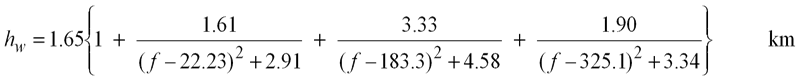
The second way is to use the scale height approximation. This models the whole atmosphere with a single set of parameters with the pressure, temperature and water vapour density taken to be those at sea level. The height of this simulated layer is called the scale height. First the attenuation vertically up to the scale height is calculated. It is not all that simple as the scale height depends on frequency. These equations should work up to about 57GHz within 10% error:
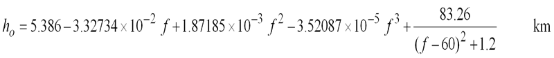
If it is a slant path we are interested in, the path length through the layer is longer. This is estimated by trigonometry with an approximation shown below based on the elevation angle, which should be limited within the range 5 - 90 degrees.
A really good model for atmospheric gas attenuation is available from the ITU-R in ITU-R P.676-6 "Attenuation by Atmospheric Gases". I have a software implementation of this on my software page.
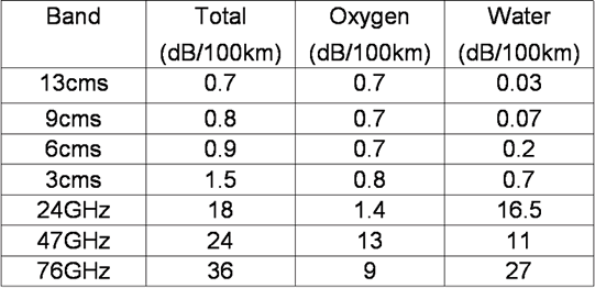
Here are some useful figures for a 100km terrestrial path at sea level with 1013 mB, 15C, Water vapour concentration 7.5g/m3
If you are calculating the gas loss for path in a duct, the recommended figure to use for the median water vapour concentration is 3g/m3
© Mike Willis May 5th, 2007