Propagation Tutorial - Variability

Variability

Most phenomena change over time and space and propagation is no different. Propagation in the troposphere is often strongly influenced by the weather and time variability is significant, for example a rain attenuation event will only happen if it is raining, this only happens for about 5% of the time in England. The resulting rain attenuation will vary according to both the rainfall rate variations within the rainstorm and through the movement of the rainstorm relative to the radio path.

Here is an example of a rain fade on a 42GHz link measured by Telenor as part of the EU 5th Framework Embrace project. It demonstrates how variations in attenuation occur over time scales of seconds to minutes.

Other metrological parameters vary as well, for example temperature and humidity vary relatively slowly with time.

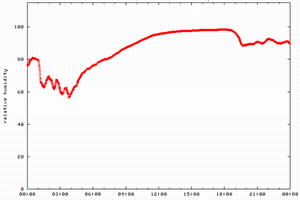
Even though the relative humidity is changing fairly slowly this event still lead to rapid changes in signal strength, as it caused significant ducting with long range enhancements and rapid multipath fading on a long range terrestrial microwave link.

Probability definitions

To describe the variability of a propagation path we can say things like:

“there is a 50% chance it will be less than this”
“it will only be this high for 10 minutes per year”
“20% of households will get a signal”
“the rate of change will only exceed X in 10% of cases”

But to plan we need some basic statistical concepts to formally describe probabilities, these will now be introduced. Some common terms that are frequently used in propagation studies are:

Annual statistics - these are the statistics of an effect measured over an “average” year

Worst Month - these are like the annual statistics but expressed for the worst month of an average year

Exceedance - the probability that some metric will be exceeded e.g. fading will exceed X dB for P% of the year

Non Exceedance - the probability that some metric will be NOT be exceeded e.g. fading will not exceed X dB for P% of the year

The Mean - The average level of a variable, often the root mean square, r.m.s. The

The Standard Deviation - A measure of how far the samples is a set of measurement deviate from their mean value

Median (Sometimes 50% value) - If you arrange all the samples of a measurement in ascending or descending order, the median is the one in the middle

Lower/upper Decile - Arrange all your measurement samples in ascending order, the bottom 10% are the lower decile, the top 10% the upper decile

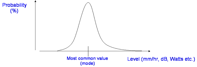
Probability Density Functions

These are very common in statistics and especially common in propagation studies. A Probability Density Function (PDF) describes the probability of a variable being at some defined value, E.g signal level

To make a PDF we first arrange the data samples into a set of value “bins” (e.g. values between 0 to 1, 1 to 2, 2 to 3, etc) and then taking the whole data set count how many samples fall into each bin. For example, say we wanted to make a PDF of the sin²(x) function from 1-10 where x is in radians.

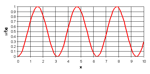
The sin²(x) function

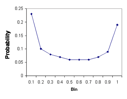
We can do this by taking samples, e.g. 100 regularly spaced samples of x between 0 and 10 and place the values of sin²(x) into 10 bins, 0-0.1, 0.1-0.2....0.9-1 as below.


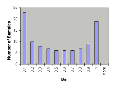The Histogram	The Probability Density Function

This result is the PDF of sin²(x). Frequently the probability axis will be as a percentage and as we are often interested in rare values it will probably also use a log scale.

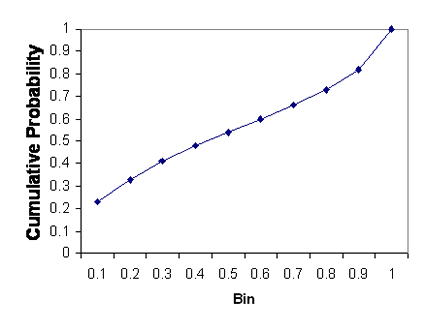
Frequently we also see the Cumulative Density Function (CDF) which is simply the cumulative sum across the PDF. You can think of a CDF as an Integral of a PDF.


The Probability Density Function	The Cumulative Density Function

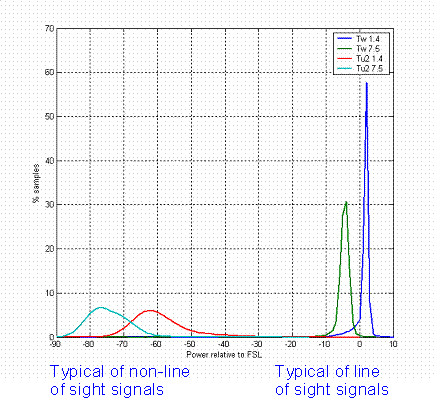
Here are some examples of real PDFs and CDFs.


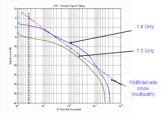A Probability Density Function The graph above is real measured data from a 70km line of sight path and a 200km trans-horizon path. The increased spread in the amplitude range of the trans-horizon data is evident.	A Cumulative Density Function The graph above is the CDF of the two line of sight signals from the plot on the left illustrating the multipath fading - note the log probability scale is along the X-axis with the signal level on the Y-axis. Plotting it this way around is just as valid.

Common Distributions

In propagation modelling, real variability of the signal is modelled as one of the "standard" distributions so that can be analytically handled. Typical standard distributions that are used are:

Normal (Gaussian) – Many measurements fonform to the Normal distribution, for example white noise
Log Normal – useful for Rain fade durations
Rayleigh – This is used in modeling urban mobile signal strengths and is a good model where there is no line of sight
Rician – This is useful for modeling rural mobile signal strength where there is line of sight plus multipath

The Normal Distribution

This is also frequently called a Gaussian distribution.

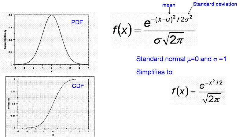
One useful feature to remember about the Normal distrivution is that 95% of the samples will lie within 2 standard deviations and 99.7% will lie within 3 standard deviations. So if you are told a model has a standard deviation of error of 8 dB, 99.7% of samples will be within ±24 dB of the mean. A standard deviation of error of 8 dB is not unusual for a mobile radio planning model.

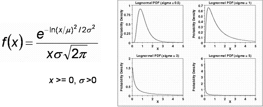
The Log-Normal Distribution

A variable x is log-normally distributed if ln(x) is normally distributed. Log normal distributions have been used to model shadowing in mobile systems.

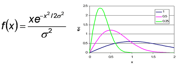
The Rayleigh Distribution

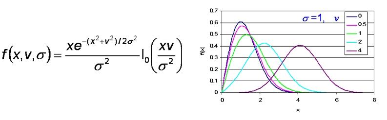
This is typical of non line of sight mobile signal levels where the power comes from many scattered paths.

The Rician Distribution

This is typical of mobile systems where there is a line of sight component as well as several strong multipath components.

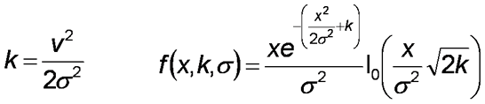
Where I_o is the first order Bessel function. Note – if v = 0, this reduces to the Rayleigh distribution.

We can re-write the equation for a Rician distribution by introducing a parameter k

k is called the “Rice Factor” and is the ratio of the power in the constant part due to the line of sight component to that in the random part due to the non-line of sight components.

Finding Data on distributions

Propagation is greatly influenced by terrain and the weather and weather data has been collected over many years. Statistics are available from the ITU SG3 for Rainfall rates, Refractivity gradients, Clouds, Wind speed, Solar activity, etc. etc. Terrain maps available from USGS for free or from OSGB if you are rich enough to pay the annual fees and can put up with the onerous usage restrictions.

The best free terrain data can be obtained from the Shuttle Radar Topography Mission (SRTM) web page. The SRTM was a joint project between the National Geospatial-Intelligence Agency (NGA) and the National Aeronautics and Space Administration (NASA).

The data was collected over a 1 arc second grid for all land areas between 60° north and 56° south latitude. For various reasons, mostly to do with “defense” global data is only available at 3 arc second resolution – but this is available for free. This is very different to OSGB data which, although better resolution is expensive and subject to strict licensing conditions.

USGS ETOPO2 Data

Unlike terrain and clutter data, there is no need to have data for climatic parameters on a fine grid of points. Point statistics of parameters at spacing of a few km are sufficient, which is fortunate as that is all that is currently available.